
Statistics & Graphics: Descriptive Statistics for Cross Sections & Panels:
Summary Measures
- Means (arithmetic, geometric), standard deviations, minima, maxima
- Medians, sample quantiles (deciles, quartiles)
- Covariances
- Correlations (Pearson, rank)
- Coefficient of concordance for a set of ranks
- Autocorrelations
- Canonical correlations
- Principal components
- Condition number for data matrices
Normality Test
- Skewness, kurtosis
- Normal-quantile plot
- Chi-squared test
Example
This is a description of Mroz’s (1987) Labor Supply Data. FAMINC is family income, stratified by KIDS, which indicates whether there are children in the household (1 = no, 2 = yes).
-------------------------------------------------------------------------
Descriptive Statistics for FAMINC
Stratification is based on KIDS
-----------------+-------------------------------------------------------
Subsample        |        Mean     Std.Dev.    Cases  Sum of wts  Missing
-----------------+-------------------------------------------------------
KIDS        =  0 |   22494.900    12174.557      229      229.00        0
KIDS        =  1 |   25144.298    11401.065      161      161.00        0
KIDS        =  2 |   22432.635    11174.183      167      167.00        0
KIDS        =  3 |   22354.590    13221.321      117      117.00        0
KIDS        =  4 |   24758.196    14798.396       56       56.00        0
KIDS        =  5 |   20004.000    11218.196       15       15.00        0
KIDS        =  6 |   20037.200    12030.108        5        5.00        0
KIDS        =  7 |    7232.000         .000        1        1.00        0
KIDS        =  8 |   12249.000     6235.268        2        2.00        0
Full Sample      |   23080.595    12190.202      753      753.00        0
-----------------+-------------------------------------------------------
Subsample        |     Minimum      Maximum    Skewness     Kurtosis
-----------------+-------------------------------------------------------
KIDS        =  0 |    1500.000    90800.000       1.615        7.675
KIDS        =  1 |    7040.000    79750.000       1.696        7.286
KIDS        =  2 |    4000.000    88000.000       1.966       10.479
KIDS        =  3 |    3777.000    96000.000       2.348       11.999
KIDS        =  4 |    2500.000    91044.000       2.261        9.981
KIDS        =  5 |    5000.000    43210.000        .490        2.386
KIDS        =  6 |   10400.000    40500.000       1.044        2.225
KIDS        =  7 |    7232.000     7232.000        .000         .000
KIDS        =  8 |    7840.000    16658.000        .000         .500
Full Sample      |    1500.000    96000.000       1.900        9.470
-----------------+-------------------------------------------------------

Quantiles
--------------------------
Percentile     FAMINC
--------------------------
Min.          1500.0
10th          11000.
20th          14027.
25th          15428.
30th          16240.
40th          18500.
Med.          20880.
60th          23300.
70th          26100.
75th          28200.
80th          30600.
90th          36872.
Max.          96000.
--------------------------
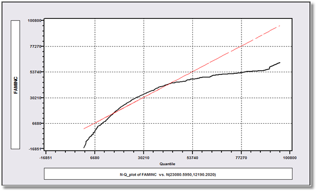
The figure shows a normal-quantile plot for the family income described above.
Data Arrangements
- Stratified data
- Weights
Analysis of Variance
- Balanced and unbalanced panels
Panel and Stratified Data
- Analysis of variance
- F test for effects
Crosstabs
- By row, column, total proportions
- Independence test
- Individual or frequency data
- Crosstabs saved as matrices
This is a cross tabulation of the labor force participation indicator against the number of children in the household for the Mroz data described above.
+-----------------------------------------------------------------+
|Cross Tabulation                                                 |
|Row variable is KIDS     (Out of range 0-49:      0)             |
|Number of Rows =  9      (KIDS     =  0 to  8)                   |
|Col variable is LFP      (Out of range 0-49:      0)             |
|Number of Cols =  2      (LFP      =  0 to  1)                   |
|Chi-squared independence tests:                                  |
|Chi-squared[   8] =   13.77724   Prob value =  .08776            |
|G-squared  [   8] =   14.29226   Prob value =  .07446            |
+-----------------------------------------------------------------+
|                    LFP                                          |
+--------+--------------+------+                                  |
|    KIDS|      0      1| Total|                                  |
+--------+--------------+------+                                  |
|       0|     93    136|   229|                                  |
|       1|     60    101|   161|                                  |
|       2|     79     88|   167|                                  |
|       3|     50     67|   117|                                  |
|       4|     29     27|    56|                                  |
|       5|     11      4|    15|                                  |
|       6|      1      4|     5|                                  |
|       7|      1      0|     1|                                  |
|       8|      1      1|     2|                                  |
+--------+--------------+------+                                  |
|   Total|    325    428|   753|                                  |
+-----------------------------------------------------------------+
Embedded Results - Transfer to Other Programs
Program results such as descriptive statistics are displayed in embedded windows that may be transported to other programs.
This is one of the National Institute of Standards and Technology test examples for benchmarking the accuracy of descriptive statistics computations.
Dataset Name:  Maryland Pick-3 Lottery
Description:   This is an observed/"real world" data set
               consisting of 218 Maryland Pick-3 Lottery values
               from September 3, 1989 to April 14, 1990 (32 weeks).
               One 3-digit random number (from 000 to 999)
               is drawn per day, 7 days per week for most
               weeks, but fewer days per week for some weeks.
               We here use this data to test accuracy
               in summary statistics calculations.
Stat Category: Univariate: Summary Statistics
Reference:     None
Data:          "Real World"
               1    Response          : y = 3-digit random number
               0    Predictors
               218  Observations
Model:         Lower Level of Difficulty
               2    Parameters        : mu, sigma
               1    Response Variable : y
               0    Predictor Variables
               y    = mu + e
                                                  Certified Values
Sample Mean                                ybar:  518.958715596330
Sample Standard Deviation (denom. = n-1)      s:  291.699727470969
Sample Autocorrelation Coefficient (lag 1) r(1):  -0.120948622967393
Number of Observations:                             218
Data: Y

READ ; Nobs = 218 ; Nvar = 1 ; Names = y ; ByVariable $
162 671 933 414 788 730 817  33 536 875 670 236 473 167 877 980 316 950
456  92 517 557 956 954 104 178 794 278 147 773 437 435 502 610 582 780
689 562 964 791  28  97 848 281 858 538 660 972 671 613 867 448 738 966
139 636 847 659 754 243 122 455 195 968 793  59 730 361 574 522  97 762
431 158 429 414  22 629 788 999 187 215 810 782  47  34 108 986  25 644
829 630 315 567 919 331 207 412 242 607 668 944 749 168 864 442 533 805
372  63 458 777 416 340 436 140 919 350 510 572 905 900  85 389 473 758
444 169 625 692 140 897 672 288 312 860 724 226 884 508 976 741 476 417
831  15 318 432 241 114 799 955 833 358 935 146 630 830 440 642 356 373
271 715 367 393 190 669   8 861 108 795 269 590 326 866  64 523 862 840
219 382 998   4 628 305 747 247  34 747 729 645 856 974  24 568 24  694
608 480 410 729 947 293  53 930 223 203 677 227  62 455 387 318 562 242
428 968

DSTAT ; Rhs = y ; AR1 $
Descriptive Statistics
--------+---------------------------------------------------------------------
Variable|       Mean       Std.Dev.     Minimum      Maximum     Cases Missing
--------+---------------------------------------------------------------------
       Y|     518.9587     291.6997          4.0        999.0      218       0
        |     Autocorrelation        -.120948623
--------+---------------------------------------------------------------------