
Statistical Analysis: Partial Effects & Oaxaca Decomposition
Partial effects can be computed automatically for any variable in any model regardless of how intricate. Oaxaca decomposition can be used for any model fit by the program, not just linear regression.
Partial Effects Reported
- Compute for all models with conditional mean functions
- Average effects
- Compute at means and at specified points
- Compute at specified strata
- List estimates and standard errors
- Compute for specified scenarios
- Appropriately account for interaction terms and nonlinearities
Dummy Variables
Partial effects distinguish between dummy variables and continuous variables. For a dummy variable, the effect is computed as the difference in the estimated probabilities with the dummy variable equal to one and zero and other variables at their means. For continuous variables, the effect is the derivative. The program also computes elasticities.
Example - Partial Effects
The following first estimates an ordered probit model for health satisfaction. The variable is coded 0-10, so there are 11 outcomes. The specification involves some nonlinearity, two interaction terms and two dummy variables, one of which is interacted with income.
HSAT* = b1 + b2*age + b3*age*age + b4*educ + b5*married + b6*female + b7*hhninc + b8*female*hhninc
-----------------------------------------------------------------------------
Ordered Probability Model
Dependent variable                 HSAT
Log likelihood function    -56863.29478
Restricted log likelihood  -57836.42214
Chi squared [   8 d.f.]      1946.25471
Significance level               .00000
McFadden Pseudo R-squared      .0168255
Estimation based on N =  27326, K =  18
Inf.Cr.AIC  = 113762.6 AIC/N =    4.163
Underlying probabilities based on Normal
--------+--------------------------------------------------------------------
        |                  Standard            Prob.      95% Confidence
    HSAT|  Coefficient       Error       z    |z|>Z*         Interval
--------+--------------------------------------------------------------------
        |Index function for probability
Constant|    2.94117***      .10632    27.66  .0000     2.73279   3.14955
     AGE|    -.03456***      .00486    -7.11  .0000     -.04409   -.02503
 AGE^2.0|     .00013**    .5466D-04     2.38  .0175      .00002    .00024
    EDUC|     .03494***      .00287    12.16  .0000      .02931    .04057
 MARRIED|     .05965***      .01548     3.85  .0001      .02932    .08999
  FEMALE|    -.19219***      .05572    -3.45  .0006     -.30140   -.08298
        |Interaction FEMALE*AGE
Intrct02|     .00361***      .00111     3.25  .0012      .00143    .00578
  HHNINC|     .28787***      .05138     5.60  .0000      .18718    .38857
        |Interaction HHNINC*FEMALE
Intrct03|    -.05835         .07056     -.83  .4083     -.19665    .07995
        |Threshold parameters for index
   Mu(1)|     .19362***      .01003    19.30  .0000      .17396    .21328
   Mu(2)|     .49967***      .01088    45.94  .0000      .47835    .52099
   Mu(3)|     .83603***      .00990    84.41  .0000      .81661    .85544
   Mu(4)|    1.10537***      .00909   121.66  .0000     1.08756   1.12317
   Mu(5)|    1.66272***      .00801   207.52  .0000     1.64702   1.67843
   Mu(6)|    1.93147***      .00774   249.57  .0000     1.91630   1.94664
   Mu(7)|    2.33904***      .00777   301.05  .0000     2.32381   2.35427
   Mu(8)|    2.99472***      .00851   351.84  .0000     2.97804   3.01140
   Mu(9)|    3.45408***      .01018   339.45  .0000     3.43414   3.47402
--------+--------------------------------------------------------------------
Note: nnnnn.D-xx or D+xx => multiply by 10 to -xx or +xx.
Note: ***, **, * ==>  Significance at 1%, 5%, 10% level.
-----------------------------------------------------------------------------
Partial effects are first computed for all variables of the probability that the health satisfaction is reported as 7.
PARTIALS ; Effects: age / educ / married / female / hhninc
         ; Outcome = 7 $

---------------------------------------------------------------------
Partial Effects  Analysis for Ordered Probit           Prob[Y =  7]
---------------------------------------------------------------------
Effects on function with respect to AGE
Results are computed by average over sample observations
Partial effects for continuous AGE      computed by differentiation
Partial effects for continuous EDUC     computed by differentiation
Partial effects for binary var MARRIED  computed by first difference
Partial effects for binary var FEMALE   computed by first difference
Partial effects for continuous HHNINC   computed by differentiation
* ==> Partial Effect for a Binary Variable
---------------------------------------------------------------------
                   Partial    Standard
(Delta method)     Effect      Error     |t|  95% Confidence Interval
---------------------------------------------------------------------
      AGE           .00037     .00005    7.10      .00027      .00048
      EDUC         -.00040     .00005    8.15     -.00050     -.00031
   *  MARRIED      -.00055     .00012    4.44     -.00079     -.00031
   *  FEMALE        .00224     .00051    4.42      .00125      .00324
      HHNINC       -.00326     .00061    5.30     -.00446     -.00205
---------------------------------------------------------------------
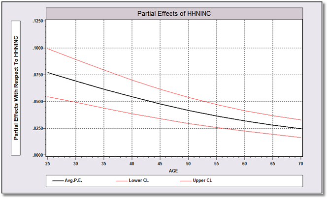
The data set is a panel observed yearly from 1984-1991. We restrict our sample to the 1991 wave, and compute average partial effects for income fixing age at 25, 30, .., 70, then plot the results as a function of age with a confidence interval around the estimated average partial effects at each age.
REJECT   ; year # 1994 $
PARTIALS ; Effects: hhninc & age = 25(5)70 ; Plot(ci)$
---------------------------------------------------------------------
Partial Effects  Analysis for Ordered Probit           Prob[Y = 10]
---------------------------------------------------------------------
Effects on function with respect to HHNINC
Results are computed by average over sample observations
Partial effects for continuous HHNINC   computed by differentiation
Effect is computed as derivative     = df(.)/dx
---------------------------------------------------------------------
df/dHHNINC         Partial    Standard
(Delta method)     Effect      Error     |t|  95% Confidence Interval
---------------------------------------------------------------------
APE. Function       .05261     .00780    6.74      .03732      .06790
AGE     = 25.00     .07677     .01140    6.73      .05443      .09912
AGE     = 30.00     .06900     .01020    6.76      .04901      .08900
AGE     = 35.00     .06139     .00905    6.78      .04365      .07914
AGE     = 40.00     .05419     .00799    6.78      .03853      .06986
AGE     = 45.00     .04758     .00704    6.76      .03379      .06137
AGE     = 50.00     .04163     .00619    6.72      .02949      .05376
AGE     = 55.00     .03637     .00546    6.66      .02566      .04708
AGE     = 60.00     .03180     .00487    6.53      .02225      .04134
AGE     = 65.00     .02786     .00442    6.30      .01920      .03653
AGE     = 70.00     .02452     .00413    5.94      .01642      .03261
Example - Oaxaca Decomposition
We continue the preceding example by decomposing the ordered probit model results for two subsamples, working and nonworking individuals. This takes two steps. In the first, the model is estimated for the two groups and (again) for the pooled sample.
ORDERED ; For [working=*,0,1]
        ; Lhs = hsat ; Rhs = one, age, age^2, educ, married, female,
                       female*age, hhninc, hhninc*female $
(We’ve omitted the three sets of estimation results.) The simple command
DECOMPOSE $
produces the decomposition.
-----------------------------------------------------
Setting up an iteration over the values of WORKING
The model command will be executed for     2 values
of this variable.  In the current sample of    3377
observations, the following counts were found:
Subsample   Observations    Subsample  Observations
WORKING  =   0       939    WORKING =   1      2438
WORKING  =****      3377
----------------------------------------------------
Actual subsamples may be smaller if missing values
are being bypassed.  Subsamples with 0 observations
will be bypassed.
-----------------------------------------------------------------
Subsample analyzed for this command is WORKING  =       0
-----------------------------------------------------------------
Subsample analyzed for this command is WORKING  =       1
-----------------------------------------------------------------
Full pooled sample is used for this iteration.
-----------------------------------------------------------------

-------------------------------------------------------------------
Decomposition of Changes in Average Functions
Model Used in Computations = Ordered Probit           Prob[Y = 10]
-------------------------------------------------------------------
               Sample is WORKING = 0         WORKING = 1     Sample
Estimates Based on                (0)                 (1)      Size
WORKING  = 0 (a)        .053819 (a,0)       .068907 (a,1)       939
WORKING  = 1 (b)        .059630 (b,0)       .083887 (b,1)      2438
Pooled   =** (*)        .056810 (*,0)       .082953 (*,1)      3377
-------------------------------------------------------------------
Wald Test of Difference in the Two Coefficient Vectors
Chi squared[ 18] =  103.2028        , P Value =  .0000
-------------------------------------------------------------------
Total Change in Function    (a,0) - (b,1) =     -.030068 ( 100.00%)
-------------------------------------------------------------------
Oaxaca    | Due to data is  (a,0) - (a,1) =     -.015088 (  50.18%)
Blinder   | Due to beta is  (a,1) - (b,1) =     -.014980 (  49.82%)
-------------------------------------------------------------------
Daymont   | Due to data is  (b,0) - (b,1) =     -.024258 (  80.68%)
Andrisani | Due to beta is  (a,0) - (b,0) =     -.005810 (  19.32%)
-------------------------------------------------------------------
Daymont   | Due to data is  (b,0) - (b,1) =     -.024258 (  80.68%)
Andrisani | Due to beta is  (a,1) - (b,1) =     -.014980 (  49.82%)
(3 Fold)  | Due to function (a,0) - (b,0) -
          |                 (a,1) - (b,1) =      .009170 ( -30.50%)
-------------------------------------------------------------------
Ransom    | Due to data is  (*,0) - (*,1) =     -.026144 (  86.95%)
Oaxaca    | Due to beta is  (a,0) - (*,0) +     -.003925 (  13.05%)
Neumark   |                 (*,1) - (b,1)
-------------------------------------------------------------------